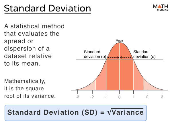
Standard deviation is a statistical measure that shows how much a group of data is spread out or dispersed from its mean value (average). A smaller standard deviation value indicates that the values are close to the mean, whereas a larger value means the dataset is spread out further from the mean. 

Mathematically, it is represented by the symbol σ (sigma) and is defined as the square root of the mean of the squares of all the values of a dataset derived from the arithmetic mean.

Based on the type of data set being analyzed and its context, there are two standard deviations: population and sample standard deviation. 

It is the measure of dispersion for an entire population. It is calculated by the formula:

${\sigma =\sqrt{\dfrac{\sum \left( x_{i}-\mu \right) ^{2}}{N}}}$

Here,

xi = Individual data values

μ = Population mean

N = Total number of data points

It is the measure of dispersion for a sample taken from a population. It is calculated by the formula:

${s=\sqrt{\dfrac{\sum \left( x_{i}-\overline{x}\right) ^{2}}{n-1}}}$

Here,

xi = Individual data values

${\overline{x}}$ = Sample mean

n = Total number of data points in the sample

Since the calculation involves squaring the differences from the mean, the standard deviation is always a positive number or 0.

Statistical data are of two types: ungrouped (raw, unorganized data) and grouped (well-organized data). 

We calculate their standard deviations as follows.

Here are the methods for determining standard deviation, depending on the type of data.

In this method, we first calculate the mean of the given data set. Next, we determine the deviation of each data point from the mean. Finally, we find the standard deviation using the formula:

${\sigma =\sqrt{\dfrac{\sum \left( x_{i}-\overline{x}\right) ^{2}}{N}}}$

Here,

xi = Individual data values

${\overline{x}}$ = Mean of the data

N = Total number of observations

Let us calculate the standard deviation for the data set 3, 2, 5, and 6

The mean is ${\overline{x}}$ = ${\dfrac{3+2+5+6}{4}=\dfrac{16}{4}=4}$

The Deviations from the Mean are 

${\left( x-\overline{x}\right) =\left( 3-4\right) ,\left( 2-4\right) ,\left( 5-4\right) ,\left( 6-4\right) =-1,-2,1,2}$

Now, taking squares of each deviation, 

(-1)2, (-2)2, (1)2, (2)2 = 1, 4, 1, 4

The sum of Squared Deviations is ${\sum \left( x-\overline{x}\right) ^{2}}$ = 1 + 4 + 1 + 4 = 10

Now, the variance = sum of squared deviations ÷ number of observations 

⇒ ${\dfrac{\sum \left( x_{i}-\overline{x}\right) ^{2}}{N}}$ = ${\dfrac{10}{4}}$ = 2.5

Thus, the standard deviation is σ = ${\sqrt{Variance}}$ = ${\sqrt{2.5}}$ ≈ 1.58

This method simplifies calculations by assuming a value close to the large set of data points as the mean, known as the assumed mean (A). The deviation from the assumed mean is calculated using the formula d = x – A. 

Finally, we find the standard deviation using the formula:

${\sigma =\sqrt{\dfrac{\sum d^{2}}{N}-\left( \dfrac{\sum d}{N}\right) ^{2}}}$

Here,

d = The deviation of each data point (x) from the assumed mean (A)

N = Total number of observations

Let us consider the previous dataset 3, 2, 5, and 6, and find the standard deviation.

Let 5 be the assumed mean A.

Now, the deviations are

d = x – A = (3 – 5), (2 – 5), (5 – 5), (6 – 5) = -2, -3, 0, 1

Now, taking the squares of the deviations,

d2 = (-2)2, (-3)2, (0)2, (1)2 = 4, 9, 0, 1

The sum of deviations is ${\sum d}$ = -2 – 3 + 0 + 1 = -4

The sum of squared deviations is ${\sum d^{2}}$ = 4 + 9 + 0 + 1 = 14

Now, the variance = sum of squared deviations ÷ number of observations 

⇒ ${\dfrac{\sum d^{2}}{N}-\left( \dfrac{\sum d}{N}\right) ^{2}}$ = ${\dfrac{14}{4}-\left( \dfrac{-4}{4}\right) ^{2}=3.5-1=2.5}$

Thus, the standard deviation is σ = ${\sqrt{Variance}}$ = ${\sqrt{2.5}}$ ≈ 1.58

In this method, we choose an arbitrary data value as the assumed mean, A, and then calculate the deviations and the step deviations.

Finally, the standard deviation of the ungrouped data is obtained by the formula:

${\sigma =i\sqrt{\left[ \dfrac{\sum \left( d’\right) ^{2}}{n}-\left( \dfrac{\sum d’}{n}\right) ^{2}\right] }}$

Here,

n = total number of data values

d = deviations of all data values = (x – A)

d’ = step deviations = ${\dfrac{d}{i}}$

i = a common factor of all d values

Just like ungrouped data, we can determine the standard deviation of grouped data by the following methods:

For grouped data, we first construct a frequency distribution. For n number of observations, say x1, x2, …, xn, and the corresponding frequencies, f1, f2, …, fn the standard deviation is calculated as follows: 

${\sigma =\sqrt{\dfrac{\sum ^{n}_{i=1}f_{i}\left( x_{i}-\overline{x}\right) ^{2}}{n}}}$

Here,

n = total frequency = ${\sum ^{n}_{i=1}f_{i}}$

${\overline{x}}$ = mean

Let us calculate the standard deviation for the data given below:

Now, calculating the midpoint (xi) and mean (${\overline{x}}$), we get

Here, ${\sum f_{i}x_{i}}$ = 75 + 200 + 350 + 315 = 940

${\sum f_{i}}$ = 5 + 8 + 10 + 7 = 30

Thus, ${\overline{x}}$ = ${\dfrac{\sum f_{i}x_{i}}{\sum f_{i}}}$ = ${\dfrac{940}{30}}$ ≈ 31.33

Now, computing all values in the formula, we get

Here, ${\sum f_{i}\left( x_{i}-\overline{x}\right) ^{2}}$ = 1333.90 + 320.56 + 134.80 + 1307.60 = 3096.86

Now, the variance is ${\dfrac{\sum f_{i}\left( x_{i}-\overline{x}\right) ^{2}}{\sum f_{i}}}$ = ${\dfrac{3096.86}{30}}$ ≈ 103.23

Thus, the standard deviation is σ = ${\sqrt{Variance}}$ = ${\sqrt{103.23}}$ ≈ 10.16

For large data sets, one of the values is chosen as the mean, and the deviation of each data set is calculated from the assumed mean.

The formula to calculate standard deviation is:

${\sigma =\sqrt{\dfrac{\sum \left( fd\right) ^{2}}{n}-\left( \dfrac{\sum fd}{n}\right) ^{2}}}$

Here,

f is the frequency of corresponding data value x 

n is the total frequency

The following table shows the number of hours students spent studying for a test. Let us calculate the standard deviation of the data using the Assumed Mean Method.

Now, calculating the midpoint (xi) for each interval, we get

Let the assumed mean A be 25

Now, computing all values in the formula, we get

Here,

n = ${\sum f_{i}}$ = 4 + 6 + 8 + 10 + 7 = 35

${\sum f_{i}d_{i}}$ = -80 – 60 + 0 + 100 + 140 = 100

${\sum f_{i}d_{i}^{2}}$ = 1600 + 600 + 0 + 1000 + 2800 = 6000

Now, the variance is ${\dfrac{\sum f_{i}d_{i}^{2}}{\sum f_{i}}-\left( \dfrac{\sum f_{i}d_{i}}{\sum f_{i}}\right) ^{2}}$ 

= ${\dfrac{6000}{35}-\left( \dfrac{100}{35}\right) ^{2}}$ ≈ 163.25

Thus, the standard deviation is σ = ${\sqrt{Variance}}$ = ${\sqrt{163.25}}$ ≈ 12.78

Here, we choose an arbitrary data value as the assumed mean, A, and then calculate the deviations and the step deviations. 

The standard deviation of grouped data by the step deviation method is given by the formula:

${\sigma =i\sqrt{\dfrac{\sum \left( fd’\right) ^{2}}{n}-\left( \dfrac{\sum fd’}{n}\right) ^{2}}}$

Here,

f = frequency of data values

n = total number of data values

d = deviations of all data values = (x – A)

d’ = step deviations = ${\dfrac{d}{i}}$

i = a common factor of all d values

A random variable can be either discrete (for countable outcomes) or continuous (for measurable outcomes). For both types, the standard deviation provides the dispersion of a set of values in a probability distribution.

To determine the standard deviation of a random variable X, we first find the difference between X and the mean or expected value (μ or E(X)) and multiply the result by the probability associated with X. Finally, we take the square root of the product. 

The standard deviation of the probability distribution of X is given by ${\sigma =\sqrt{\sum \left[ \left( x-\mu \right) ^{2}\cdot P\left( x\right) \right] }}$

However, there is a shortcut to find the standard deviation of random variables, which is done by the formula: 

${\sigma =\sqrt{E\left( X^{2}\right) -\left[ E\left( X\right) \right] ^{2}}}$ or ${\sigma =\sqrt{\sum \left[ x^{2}\cdot P\left( x\right) \right] -\mu ^{2}}}$

For a continuous random variable X with a probability density function f(x), the standard deviation is calculated as

${\sigma =\sqrt{\int ^{\infty }_{-\infty }\left( x-\mu \right) ^{2}f\left( x\right) dx}}$

The method can be applied to discrete or continuous random variables, using either a probability function or a probability density function, as appropriate.

Standard deviation varies based on the type of probability distribution:

Since the mean is 0, the standard deviation is 1.

The standard deviation is given by: 

σ = ${\sqrt{npq}}$

Here, 

μ = np is the mean 

n is the number of trials 

p is the probability of success

q = 1 – p is the probability of failure

The standard deviation is given by: 

σ = ${\sqrt{\lambda t}}$

Here,

λ is the average number of successes in an interval of time t

Example 1: There are 25 students in a class. A few students were selected randomly, and their test scores were recorded as follows: 67, 74, 81, 69, 85. Calculate the standard deviation of their scores.

Given sample size n = 25

Calculating the sample mean, we get 

${\overline{x}}$ = ${\dfrac{67+74+81+69+85}{5}}$ = 75.2

Calculating the deviations from the mean and their squares, we get

Now, adding up all the squared deviations, we get

${\sum \left( x_{i}-\overline{x}\right) ^{2}}$ = 67.24 + 1.44 + 33.64 + 38.44 + 96.04 = 236.8

Calculating the variance, we get

Variance = ${\dfrac{\sum \left( x_{i}-\overline{x}\right) ^{2}}{n-1}}$ = ${\dfrac{236.8}{5-1}}$ = 59.2

Thus, the standard deviation is σ = ${\sqrt{Variance}}$ = ${\sqrt{59.2}}$ ≈ 7.7